[LSTF] Informer: Beyond Efficient Transformer for Long Sequence Time-Series Forecasting

LSTF(Long Sequence Time-Series Forecasting)이란?

LSTF Journal

LSTF DSBA 동영상

Transformer에서는 LSTF에 직접 적용하기 어려운 문제(quadratic time complexity(Quadratic한 연산 복잡도), high memory usage(높은 메모리 사용량), and inherent limitation of the encoder-decoder architecture(인코더-디코더 모델의 step-by-step inference 속도 문제))를 해결하기 위해 Informer라는 효율적인 LSTF기반 모델을 설계했다.

1) ProbSparse Self-Attention 매커니즘으로 시간복잡도와 메모리 사용량 효율 향상

2) Self-Attention distilling기법은 cascading layer input을 절반으로 줄여 long time-series sequence 를 효율적으로 처리

3) Generative style decoder를 통해 하나의 forward step만으로 long time-series sequence 예측 가능

Intorduction

과거의 시계열 예측은 48point이하를 예측하는 단기적인 문제(Short-Term)를 다뤄왔다.

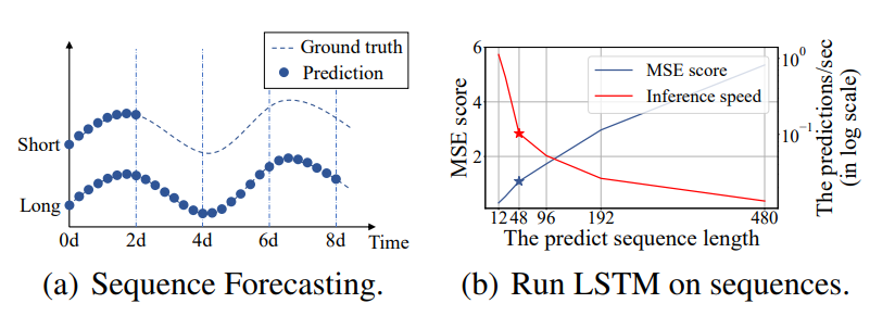
(b)에서는 predict sequece length 48부터 MSE는 높아지고 Inference speed(추론 속도)는 급격하게 떨어진다.

최근 Transformer모델은 RNN모델보다 장거리 의존성 포착 성능이 우수하나 (b)조건에서는 떨어진다.

• (b)가 떨어지는 원인
  • The quadratic computation of self-attention: canonical dot-product은 시간복잡도와 메모리 사용량을 \(O(L^2)\) 소요
  • The memory bottleneck in stacking layers for long inputs: J개 encoder-decoder layer를 쌓으면 \(O(j·L^2)\) 이 되어 long sequece input을 받을 때 모델 확장성 제한
  • The speed plunge in predicting long outputs: Vanilla Transformer의 Dynamic decording은 RNN보다 step-by-step inference가 느림

Preliminary

LSTF Problem 정의

• Input:
  \(X_t = \left\{x^t_1, ..., x^t_{L_x} \mid x^t_i \in \mathbb{R}^{dx}\right\}\)
• Output:
  \(Y_t = \left\{y^t_1, ..., y^t_{L_y} \mid y^t_i \in \mathbb{R}^{dy}\right\}\)

Encoder-decoder architecture

• 많은 Encoder-decoder 구조는 input representation \(X^t\) → Encoder → hidden representation \(H^t\) 생성 → decoder →output representation \(Y^t\) 를 수행함

• Informer는 순차적 예측이 아닌 한번의 forward step으로 예측 진행

Input Representation

• uniform input representation은 global positional context와 local temporal context를 향상시킴

 

• RNN: recurrnet structure로 time-series pattern을 포착하며 time stamps에 의존하지 않음
• vanilla transformer: point-wise self-attention을 사용하고, time stamps를 local positional context의 역할을 함

 

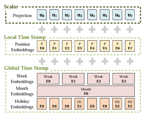
• Scaler: input \(x^t_i\) 을 \(d_{model}\) 차원으로 projection시킨 값
• Local Time Stamp: 일반적인 transformer의 Positional Encoder방식으로 fixed값 사용
• Gloabl Time Stamp: 학습 가능한(learnable) embedding 사용

Methodology

Efficient Self-attention Mechanism

self-attention: \(\mathcal{A}(\mathbf{Q}, \mathbf{K}, \mathbf{V}) = \mathrm{Softmax}\left(\frac{\mathbf{Q}\mathbf{K}^{\top}}{\sqrt{d}}\right)\mathbf{V}\)

• the \(i\)-thquery’sattention: \(\mathcal{A}(\mathbf{q}_i, \mathbf{K}, \mathbf{V}) = \sum_j \frac{k(\mathbf{q}_i, \mathbf{k}_j)}{\sum_l k(\mathbf{q}_i, \mathbf{k}_l)}\mathbf{v}_j = \mathbb{E}_{p(\mathbf{k}_j|\mathbf{q}_i)}[\mathbf{v}_j]\,, \tag{1}\)

• self-attention은 \(p(\mathbf{k}_j|\mathbf{q}_i) = \frac{k(\mathbf{q}_i, \mathbf{k}_j)}{\sum_l k(\mathbf{q}_i, \mathbf{k}_l)}\) 확률 계산을 기반으로 출력을 얻음 -> 예측 성능을 향상할 떄 주요 단점으로 작용

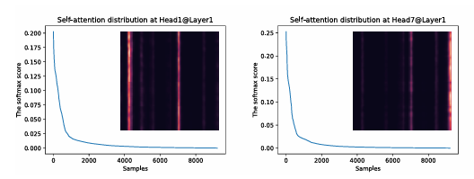
• The“sparsity”self-attentionscore

  • 긴 꼬리 분포를 형성하고 소수의 dot-product pairs이 대부분의 attention 차지하고, trivial attention을 생성함

QuerySparsityMeasurement

\(p(k_j|q_i)\) 가 균등 분포 \(q(k_j|q_i) = 1/L_K\) 에 가까워지면 self-attention은 trivial값들의 합이 되어 input에 의미가 없어짐 (정보 손실)

• solution
  • 분포 p와 q를 Kullback-Leibler distance로 측정하여 likeness 측정
  • \[KL(q\|p)= \ln \sum_{l=1}^{L_K} e^{\mathbf{q}_i \mathbf{k}_l^\top / \sqrt{d}} - \frac{1}{L_K} \sum_{j=1}^{L_K} \mathbf{q}_i \mathbf{k}_j^\top / \sqrt{d} - \ln L_K\]
  • 첫번째 항: log-sum-exp
  • $i$ 번째 qeury sparsity 측정값 \(M(\mathbf{q}_i, \mathbf{K}) =\ln \sum_{j=1}^{L_K} e^{\mathbf{q}_i \mathbf{k}_j^\top / \sqrt{d}}- \frac{1}{L_K} \sum_{j=1}^{L_K} \mathbf{q}_i \mathbf{k}_j^\top / \sqrt{d}\)
  • 두번째 항: arithmetic mean(산술평균)
• M이 클 수록 attention probability p는 다양한 확률 값을 갖고, 유의미한 dot-product pairs를 가질 가능성이 높음

ProbSparseSelf-attention

• 쿼리 희소성 측정값 \(M(\mathbf{q}_i, \mathbf{K})\)을 이용해 상위 u개 쿼리만을 선택(Top-u)
• \[\mathcal{A}(\mathbf{Q}, \mathbf{K}, \mathbf{V}) = \mathrm{Softmax}\left(\frac{\overline{\mathbf{Q}}\, \mathbf{K}^{\top}}{\sqrt{d}}\right)\mathbf{V}\]
• \(\overline{\mathbf{Q}}\) 는 희소 행렬(쿼리 행렬과 동일한 크기)이지만, 희소성 측정값 \(M(\mathbf{q}, \mathbf{K})\)을 기준으로 Top-u 쿼리만 포함

• 샘플링 계수 \(c\)에 의해 \(u = c \cdot \ln L_Q\)로 설정하며, ProbSparse self-attention은 qeury-key pairs 계산에서 \(O(ln L_Q)\)필요하므로 레이어 메모리 사용량은 \(O(L_K \ln L_Q)\)

• 그러나 모든 쿼리 값을 탐색하여 측정값 \(M(\mathbf{q}_i, \mathbf{K})\)을 구하려면 각 dot-product pairs을 계산해야 하므로 계산량이 \(O(L_Q L_K)\)로 많고, LSE는 수치적 불안정성 문제까지 있을 수 있어 근사 방법을 제안

Lemma 1

• 각 쿼리 \(\mathbf{q}_i \in \mathbb{R}^d\)와 키 \(\mathbf{k}_j \in \mathbb{R}^d\)가 키 집합 \(\mathbf{K}\)에 있을 때, 다음과 같은 경계(bound)가 성립

\[\ln L_K \leq M(\mathbf{q}_i, \mathbf{K}) \leq \max_j\left\{ \frac{\mathbf{q}_i \mathbf{k}_j^\top}{\sqrt{d}} \right\} - \frac{1}{L_K} \sum_{j=1}^{L_K} \frac{\mathbf{q}_i \mathbf{k}_j^\top}{\sqrt{d}} + \ln L_K\]

• \(\mathbf{q}_i \in \mathbf{K}\)인 경우에도 위 식이 성립

---

\[\overline{M}(\mathbf{q}_i, \mathbf{K}) = \max_j \left\{ \frac{\mathbf{q}_i \mathbf{k}_j^\top}{\sqrt{d}} \right\} - \frac{1}{L_K} \sum_{j=1}^{L_K} \frac{\mathbf{q}_i \mathbf{k}_j^\top}{\sqrt{d}}\]

• Top-u 범위는 Proposition 1의 경계 이완(bounding relaxation)을 기반으로 근사적으로 유지
• 롱테일 분포에서는 일부 dot-product 쌍만 샘플링하여 \(\overline{M}(\mathbf{q}_i, \mathbf{K})\)를 계산(나머지 값은 0으로 처리).
• Sparse Top-u는 \(\mathbf{Q}\)에서 선택
• \(\overline{M}(\mathbf{q}_i, \mathbf{K})\)는 값이 0 근처일 때도 수치적으로 안정적.
• 실제 self-attention에서 쿼리/키 길이가 같으면,
  • 시간 복잡도 및 공간 복잡도: \(\mathcal{O}(L \ln L)\).

Encoder: Allowing for Processing Longer Sequential Inputs under the Memory Usage Limitation

• 긴 순차 입력의 장기 의존성을 효율적으로 추출하면서 메모리 사용량을 효과적으로 통제하는 인코더 구조 설계
• 입력 \(x^t\)는
  \(X_{\text{en}}^t \in \mathbb{R}^{L_x \times d_{\text{model}}}\)
  형태의 행렬로 전처리되어 인코더에 투입됨

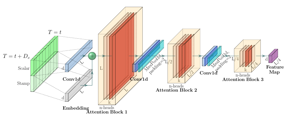
Self-attention Distilling

• 중요한 특징만 남기고, 각 레이어에 집중된 셀프어텐션 피처 맵을 전달하는 distilling 연산 수행 시간 축을 절반으로 줄이며, 각 레이어의 n-head 어텐션 결과를 압축

• \[X^{t}_{j+1} = \text{MaxPool}\Bigl( \text{ELU}\bigl( \text{Conv1d}( [X^t_{j}]_{AB} ) \bigr) \Bigr)\]
• \(\mathrm{Conv1d}\): 1차원 합성곱(커널 크기 3)
• \(\mathrm{ELU}\): 활성화 함수 (Clevert et al., 2016)
• \(\mathrm{MaxPool}\): 시간 축 시퀀스를 절반으로 다운샘플링
• \([\,\cdot\,]_{AB}\): 어텐션 블록 (Multi-head ProbSparse Self-attention + Conv1d)

MaxPooling 레이어를 활용해 시퀀스를 절반 길이로 다운샘플링 하므로, 스택이 쌓일 때마다 전체 메모리 요구량이 \(\mathcal{O}((2-\epsilon)L\log L)\)로 줄어듬

Decoder: Generating Long Sequential Outputs Through One Forward Procedure

• 표준 디코더 구조(참조: Vaswani et al., 2017)를 사용하며,
  2개의 multi-head attention layer로 구성됨.

• 작동 원리:

  • 디코더 입력 벡터: \(X_{\text{de}}^t = \mathrm{Concat}(X_{\text{token}}^t, X_0^t) \in \mathbb{R}^{(L_{\text{token}} + L_y) \times d_{\text{model}}}\)
    • \(X_{\text{token}}^t\): 시작 토큰 (Shape: \(\mathbb{R}^{L_\text{token} \times d_\text{model}\)))
    • \(X_0^t\): 타깃 시퀀스 자리표시(Shape: \(\mathbb{R}^{L_y \times d_\text{model}\))), 실제 값은 0으로 세팅
  • Masked multi-head attention에서 ProbSparse self-attention 사용(마스킹: \(-\infty\)로 설정해 미래 정보 차단)
  • fully-connected 레이어가 마지막 예측값을 산출하며,
    outsize \(d_y\)는 uni/multivariate 예측 타입에 따라 결정

---

Generative Inference

• 핵심 아이디어
  • NLP의 “dynamic decoding”과 유사하게 시작 토큰을 빠르게 적용하여, 한 번의 순방향 연산으로 전체 타깃 시퀀스를 생성함
  • 특정 토큰만 고르는 대신, 입력 시퀀스 중 최근 구간(예: 타깃 예측 바로 전 5일)을 ‘start token’으로 사용
    • 예시: 168 포인트(7일 온도 예측)라면, 이전 5일 데이터를 \(X_{-5d}\)로 선택
  • 생성형 인퍼런스 디코더 입력: \(X_{\text{de}} = \{ X_{-5d}, X_0 \}\)
    • \(X_0\): 타깃시퀀스의 타임스탬프, 즉 해당 주의 맥락 정보
  • 디코더는 동적 디코딩 대신, 전체 예측값을 한 번의 forward 연산으로 출력
    → 전통적인 encoder-decoder 방식보다 더 빠름

---

Loss function

• 예측 손실은 MSE(Minimum Square Error)로 계산
  • 디코더 모든 출력에 대해 MSE를 누적하여 학습