[Data Analysis] 차원축소 기반 이상 탐지

PCA, t-SNE을 이용한 이상탐지 구현해보기

게시 2025/03/04

By 황병현

7 분읽는 시간

PCA 이상 탐지

PCA(Principal Component Analysis)란 변수에서 가장 가까운 초평면을 구한 다음, 초평면을 투영(Projection)하여 차원을 축소하는 기법입니다.

AutoEncoder의 작동원리인 정보를 압축하고 복원하면서 데이터를 실제와 가깝게 복원시키기 위해 정상 데이터의 패턴을 학습하고 비 정상인 데이터는 복원 패턴을 배우지않으며 비정상인 데이터를 찾는 것과 비슷합니다.

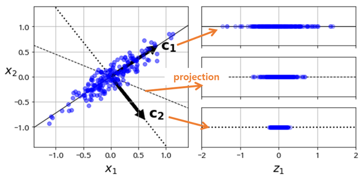
PCA는 다음과 같은 단계로 이루어집니다.

학습 데이터셋에서 분산이 최대인 축(axis)을 찾습니다.
이렇게 찾은 첫번째 축과 직교(orthogonal)하면서 분산이 최대인 두 번째 축을 찾습니다.
첫 번째 축과 두 번째 축에 직교하고 분산을 최대한 보존하는 세 번째 축을 찾습니다.
1~3과 같은 방법으로 데이터셋의 차원(특성 수)만큼의 축을 찾습니다.

장점
- 선택한 변수들의 해석이 용이함
- 고차원에서 저차원으로 줄일 수 있음
단점
- 변수간 상관관계를 고려하기 어려움
- 추출된 변수 해석 어려움

주의 : PCA는 정규화를 필수로 요구합니다.(아래 데이터는 정규화가 진행되어있습니다.)

  
from sklearn.decomposition import PCA
import pandas as pd

data = pd.read_csv('creditcard.csv')
data

	Time	V1	V2	V3	V4	V5	V6	V7	V8	V9	...	V21	V22	V23	V24	V25	V26	V27	V28	Amount	Class
0	0.0	-1.359807	-0.072781	2.536347	1.378155	-0.338321	0.462388	0.239599	0.098698	0.363787	...	-0.018307	0.277838	-0.110474	0.066928	0.128539	-0.189115	0.133558	-0.021053	149.62	0
1	0.0	1.191857	0.266151	0.166480	0.448154	0.060018	-0.082361	-0.078803	0.085102	-0.255425	...	-0.225775	-0.638672	0.101288	-0.339846	0.167170	0.125895	-0.008983	0.014724	2.69	0
2	1.0	-1.358354	-1.340163	1.773209	0.379780	-0.503198	1.800499	0.791461	0.247676	-1.514654	...	0.247998	0.771679	0.909412	-0.689281	-0.327642	-0.139097	-0.055353	-0.059752	378.66	0
3	1.0	-0.966272	-0.185226	1.792993	-0.863291	-0.010309	1.247203	0.237609	0.377436	-1.387024	...	-0.108300	0.005274	-0.190321	-1.175575	0.647376	-0.221929	0.062723	0.061458	123.50	0
4	2.0	-1.158233	0.877737	1.548718	0.403034	-0.407193	0.095921	0.592941	-0.270533	0.817739	...	-0.009431	0.798278	-0.137458	0.141267	-0.206010	0.502292	0.219422	0.215153	69.99	0
...	...	...	...	...	...	...	...	...	...	...	...	...	...	...	...	...	...	...	...	...	...
284802	172786.0	-11.881118	10.071785	-9.834783	-2.066656	-5.364473	-2.606837	-4.918215	7.305334	1.914428	...	0.213454	0.111864	1.014480	-0.509348	1.436807	0.250034	0.943651	0.823731	0.77	0
284803	172787.0	-0.732789	-0.055080	2.035030	-0.738589	0.868229	1.058415	0.024330	0.294869	0.584800	...	0.214205	0.924384	0.012463	-1.016226	-0.606624	-0.395255	0.068472	-0.053527	24.79	0
284804	172788.0	1.919565	-0.301254	-3.249640	-0.557828	2.630515	3.031260	-0.296827	0.708417	0.432454	...	0.232045	0.578229	-0.037501	0.640134	0.265745	-0.087371	0.004455	-0.026561	67.88	0
284805	172788.0	-0.240440	0.530483	0.702510	0.689799	-0.377961	0.623708	-0.686180	0.679145	0.392087	...	0.265245	0.800049	-0.163298	0.123205	-0.569159	0.546668	0.108821	0.104533	10.00	0
284806	172792.0	-0.533413	-0.189733	0.703337	-0.506271	-0.012546	-0.649617	1.577006	-0.414650	0.486180	...	0.261057	0.643078	0.376777	0.008797	-0.473649	-0.818267	-0.002415	0.013649	217.00	0

284807 rows × 31 columns

  
# Time, Amomunt 변수 제거
data.drop(['Time', 'Amount'], axis=1, inplace=True)

  
pca = PCA()
pca.fit(data.drop(['Class'], axis=1))

PCA()

In a Jupyter environment, please rerun this cell to show the HTML representation or trust the notebook.
On GitHub, the HTML representation is unable to render, please try loading this page with nbviewer.org.

  
# 차원축소 주성분 갯수 확인
features = range(pca.n_components_)
feature_df=pd.DataFrame(data=features,columns=['pc_feature'])

# 설명력 확인
variance_df=pd.DataFrame(data=pca.explained_variance_ratio_,columns=['variance'])
variance_df["cumulative_variance"] = variance_df["variance"].cumsum()

# 전체 분산에 95% 이상 설명 가능(feature 22개 채택)
pc_feature_df=pd.concat([feature_df,variance_df],axis=1)
pc_feature_df

	pc_feature	variance	cumulative_variance
0	0	0.124838	0.124838
1	1	0.088729	0.213567
2	2	0.074809	0.288376
3	3	0.065231	0.353608
4	4	0.061990	0.415598
5	5	0.057756	0.473354
6	6	0.049799	0.523153
7	7	0.046417	0.569570
8	8	0.039275	0.608845
9	9	0.038579	0.647423
10	10	0.033901	0.681325
11	11	0.032488	0.713812
12	12	0.032233	0.746045
13	13	0.029901	0.775946
14	14	0.027262	0.803208
15	15	0.024984	0.828192
16	16	0.023473	0.851665
17	17	0.022860	0.874526
18	18	0.021563	0.896088
19	19	0.019339	0.915427
20	20	0.017556	0.932983
21	21	0.017137	0.950120
22	22	0.012689	0.962809
23	23	0.011936	0.974745
24	24	0.008842	0.983587
25	25	0.007567	0.991153
26	26	0.005301	0.996455
27	27	0.003545	1.000000

  
import matplotlib.pyplot as plt
import seaborn as sns
%matplotlib inline

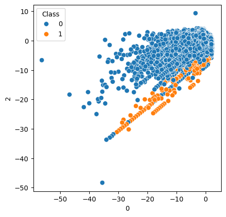
x = data.drop(['Class'], axis=1)
y = data['Class']

pca = PCA(n_components=22)
x_pca = pca.fit_transform(x)

pc_df=pd.DataFrame(x_pca,columns=[f'{i}' for i in range(22)]).reset_index(drop=True)
pc_df=pd.concat([pc_df,y],axis=1)

plt.rcParams['figure.figsize'] = [5, 5]
sns.scatterplot(data=pc_df,x='0',y='2',hue=y, legend='brief', s=50, linewidth=0.5);

t-SNE 이상 탐지

t-SNE(t-distributed Stochastic Neighbor Embedding)는 비선형 차원 축소 기법으로 t-분포를 사용하여 데이터 유사도를 계산하여 유사도가 낮은 데이터는 멀리 떨어뜨려 거리를 최대한 보존합니다.

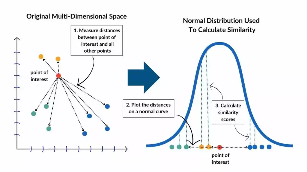
🔹 t-SNE 동작 과정

고차원 공간에서 데이터 포인트 간 확률적 유사도 계산
저차원 공간에서 랜덤하게 초기화된 점들의 분포 생성
저차원 공간에서도 유사한 확률 분포를 유지하도록 위치 조정
최적화 수렴 후 최종 시각화 결과 생성

장점
- PCA 대비 클러스터링을 발견하기 쉬움
- 비선형 관계의 데이터를 군집화 가능
단점
- 대량의 데이터에서 속도가 느림 (O(n²) 복잡도)
- 매번 돌릴 때마다 다른 시각화 결과가 도출

  
from sklearn.manifold import TSNE
from sklearn.model_selection import train_test_split

# 데이터 갯수 줄이기(약 30만개의 데이터를 넣으면 시간이 오래걸립니다.)
df_reduced, _ = train_test_split(data, train_size=0.03, stratify=data['Class'], random_state=42)

df_reduced['Class'].value_counts()

	count
Class
0	8529
1	15

dtype: int64

  
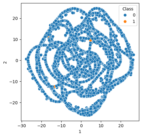
# t-SNE 2차원 축소(t-SNE는 4차원 이상으로 변환할 수 없습니다.)
tsne_np = TSNE(n_components = 3, random_state=42).fit_transform(df_reduced.drop(['Class'], axis=1))

tsne_df = pd.DataFrame(tsne_np, columns = [f'{i}' for i in range(3)])
tsne_df

	0	1	2
0	-2.370444	-12.131145	19.459503
1	-18.261276	0.444234	-0.662202
2	5.660702	-2.703253	-14.699653
3	0.748979	4.191403	4.901437
4	-6.995453	-8.831751	-17.670755
...	...	...	...
8539	11.484577	18.109447	-3.144772
8540	11.609701	14.841992	8.453781
8541	-6.828044	-9.141667	-16.934467
8542	2.451750	-3.080299	-7.047642
8543	7.451354	-21.366283	-0.024991

8544 rows × 3 columns

  
import matplotlib.pyplot as plt
import seaborn as sns
%matplotlib inline

y = df_reduced['Class'].reset_index(drop=True)

plt.rcParams['figure.figsize'] = [5, 5]
sns.scatterplot(data=tsne_df,x='1',y='2',hue=y, legend='brief', s=50, linewidth=0.5);

참고자료

Data Analysis, Anomaly Detection

Data Analysis Anomaly Detection

PCA 이상 탐지

t-SNE 이상 탐지

인기 태그