[Data Analysis] 트리 & 분류 기반 이상 탐지

트리 및 분류 기반 이상탐지를 진행하였습니다.

게시 2025/02/24

By 황병현

9 분읽는 시간

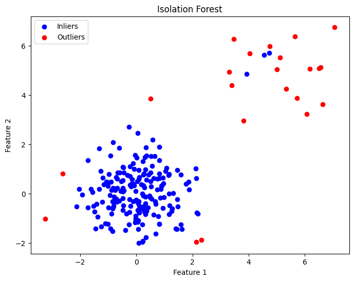
Isolation Forest 이상 탐지

임의의 변수에 임의의 값을 사용하여 split해 내가 isolation하고 싶은 객체가 존재하지 않는 부분을 버리는 방식

특정 한 개체가 isolation 되는 leaf 노드(terminal node)까지의 거리를 anomaly score로 정의
그 평균거리(depth)가 짧을 수록 anomaly score는 높아짐
split이 적으면 anomaly score은 커짐
split이 많으면 anomaly score은 작아짐

Anomaly Score 계산

Anomaly Score는 다음과 같은 수식으로 계산된다.:

여기서 E(h(x))는 각 데이터 포인트의 평균 경로 길이, c(n)은 전체 데이터의 평균 경로 길이를 보정하는 상수

트리 높이의 제한을 엄격하게 줄때( h l i m = 1 ) 정상분포와 비정상분포의 스코어가 유사함
트리 높이의 제한을 덜 줄때( h l i m = 6 ) 정상분포(0.45)와 비정상분포(0.55)의 스코어가 적절히 구분되어 표기됨
장점
- 군집기반 이상탐지 알고리즘에 비해 계산량이 매우 적음(smapling을 사용해서 트리를 생성)
- 이상치가 포함되지 않아도 동작함
- 비지도 학습이 가능하다
단점
- 수직과 수평으로 분리하기 때문에 잘못된 scoring이 발생할 수 있음

  
from sklearn.ensemble import IsolationForest

import pandas as pd
import numpy as np

  
np.random.seed(42)
n_samples = 200
n_features = 2

X_normal = np.random.normal(loc=[0,0], scale=[1,1], size=(n_samples, n_features))

X_outlier = np.random.normal(loc=[5, 5], scale=[1, 1], size=(int(n_samples * 0.1), n_features))

X = np.vstack((X_normal, X_outlier))

  
# contamination : 이상치의 비율 설정(default = 'auto')
iforest = IsolationForest(contamination=0.1, random_state=42)
iforest.fit(X)

# 예측
y_pred = iforest.predict(X)

  
import matplotlib.pyplot as plt
%matplotlib inline

# 이상치와 정상 데이터를 색상으로 구분하여 시각화
plt.figure(figsize=(8, 6))
plt.scatter(X[y_pred == 1, 0], X[y_pred == 1, 1], c='blue', label='Inliers')
plt.scatter(X[y_pred == -1, 0], X[y_pred == -1, 1], c='red', label='Outliers')
plt.title('Isolation Forest')
plt.xlabel('Feature 1')
plt.ylabel('Feature 2')
plt.legend()
plt.show()

Extended Isolation Forest 이상 탐지

Isolation Forest기반으로 확장된 알고리즘으로 수직과 평면으로 분기를 나누는 것을 넘어 초평면을 사용하여 데이터를 나누는 방식

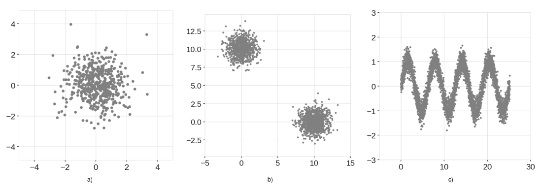
위 데이터를 분할하는데 기존의 isolation은 수직과 수평으로 분할하면 아래와 같다.

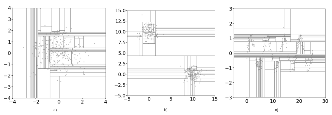
이는 수직과 수평이 교차하여 데이터가 없는 곳에 낮은 이상 점수 영역을 만드는 문제가 발생하게 된다.

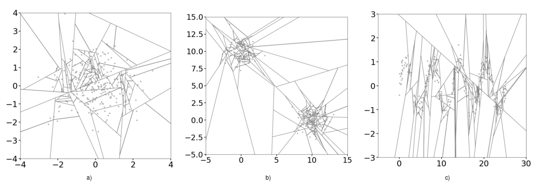
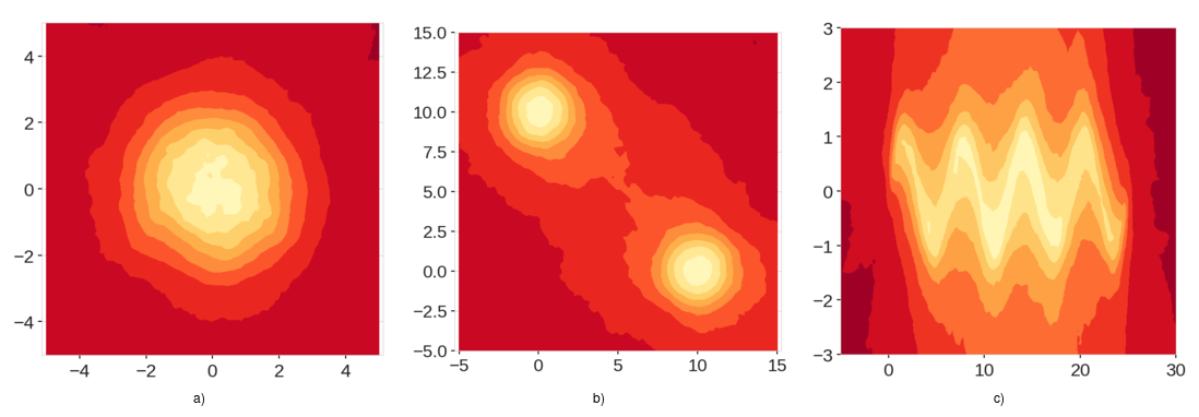
이에 Extended Isolation Forest는 분기 과정을 모든 방향으로 발생시키도록하여 지역을 훨씬 더 균일하게 나뉘게 할 수 있었으며, 데이터가 없는 곳에 이상 점수 영역을 만들지 않게 만들 수 있게 되었다.

장점
- 복잡한 데이터 구조에서 isolation forest보다 잘 탐지함
- isolation forest와 비슷하게 속도저하가 없음
단점
- hyper parameter를 많이 조정해야 함.

  
import h2o
from h2o.estimators import H2OExtendedIsolationForestEstimator

# H2O 초기화
h2o.init()

Checking whether there is an H2O instance running at http://localhost:54321..... not found.
Attempting to start a local H2O server...
  Java Version: openjdk version "11.0.26" 2025-01-21; OpenJDK Runtime Environment (build 11.0.26+4-post-Ubuntu-1ubuntu122.04); OpenJDK 64-Bit Server VM (build 11.0.26+4-post-Ubuntu-1ubuntu122.04, mixed mode, sharing)
  Starting server from /usr/local/lib/python3.11/dist-packages/h2o/backend/bin/h2o.jar
  Ice root: /tmp/tmp_xjhwin6
  JVM stdout: /tmp/tmp_xjhwin6/h2o_unknownUser_started_from_python.out
  JVM stderr: /tmp/tmp_xjhwin6/h2o_unknownUser_started_from_python.err
  Server is running at http://127.0.0.1:54321
Connecting to H2O server at http://127.0.0.1:54321 ... successful.
Warning: Your H2O cluster version is (3 months and 22 days) old.  There may be a newer version available.
Please download and install the latest version from: https://h2o-release.s3.amazonaws.com/h2o/latest_stable.html


H2O_cluster_uptime:	06 secs
H2O_cluster_timezone:	Etc/UTC
H2O_data_parsing_timezone:	UTC
H2O_cluster_version:	3.46.0.6
H2O_cluster_version_age:	3 months and 22 days
H2O_cluster_name:	H2O_from_python_unknownUser_vpnhj2
H2O_cluster_total_nodes:	1
H2O_cluster_free_memory:	3.170 Gb
H2O_cluster_total_cores:	2
H2O_cluster_allowed_cores:	2
H2O_cluster_status:	locked, healthy
H2O_connection_url:	http://127.0.0.1:54321
H2O_connection_proxy:	{"http": null, "https": null, "colab_language_server": "/usr/colab/bin/language_service"}
H2O_internal_security:	False
Python_version:	3.11.11 final

  
h2o_df = h2o.import_file("https://raw.github.com/h2oai/h2o/master/smalldata/logreg/prostate.csv")

predictors = ["AGE","RACE","DPROS","DCAPS","PSA","VOL","GLEASON"]

# Extended Isolation Forest 모델 생성 및 학습
eif = H2OExtendedIsolationForestEstimator(model_id = "eif.hex",
                                          ntrees = 100,
                                          sample_size = 256,
                                          extension_level = len(predictors) - 1)

eif.train(x=predictors, training_frame=h2o_df)

# 예측
y_pred = eif.predict(h2o_df).as_data_frame()

Parse progress: |████████████████████████████████████████████████████████████████| (done) 100%
extendedisolationforest Model Build progress: |██████████████████████████████████| (done) 100%
extendedisolationforest prediction progress: |███████████████████████████████████| (done) 100%


/usr/local/lib/python3.11/dist-packages/h2o/frame.py:1983: H2ODependencyWarning: Converting H2O frame to pandas dataframe using single-thread.  For faster conversion using multi-thread, install polars and pyarrow and use it as pandas_df = h2o_df.as_data_frame(use_multi_thread=True)

  warnings.warn("Converting H2O frame to pandas dataframe using single-thread.  For faster conversion using"

  
anomaly_score = y_pred["anomaly_score"]

# 데이터셋과 이상치 점수 결합
prostate_df = h2o_df.as_data_frame()
prostate_df['anomaly_score'] = anomaly_score

/usr/local/lib/python3.11/dist-packages/h2o/frame.py:1983: H2ODependencyWarning: Converting H2O frame to pandas dataframe using single-thread.  For faster conversion using multi-thread, install polars and pyarrow and use it as pandas_df = h2o_df.as_data_frame(use_multi_thread=True)

  warnings.warn("Converting H2O frame to pandas dataframe using single-thread.  For faster conversion using"

  
prostate_df.head(5)

	ID	AGE	RACE	DPROS	DCAPS	PSA	VOL	GLEASON	anomaly_score
0	1	65	1	2	1	1.4	0.0	6	0.379427
1	2	72	1	3	2	6.7	0.0	7	0.371727
2	3	70	1	1	2	4.9	0.0	6	0.380674
3	4	76	2	2	1	51.2	20.0	7	0.492321
4	5	69	1	1	1	12.3	55.9	6	0.449620

  
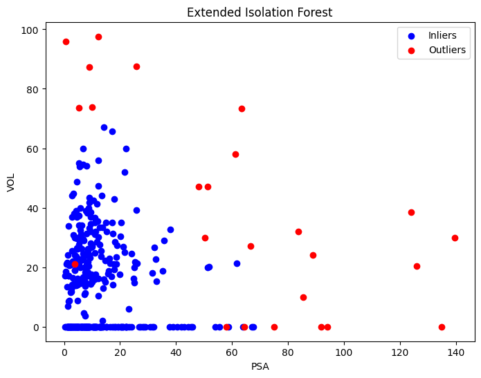
plt.figure(figsize=(8, 6))
plt.scatter(prostate_df.loc[prostate_df['anomaly_score'] < 0.5, 'PSA'], prostate_df.loc[prostate_df['anomaly_score'] < 0.5, 'VOL'], c='blue', label='Inliers')
plt.scatter(prostate_df.loc[prostate_df['anomaly_score'] >= 0.5, 'PSA'], prostate_df.loc[prostate_df['anomaly_score'] >= 0.5, 'VOL'], c='red', label='Outliers')
plt.title('Extended Isolation Forest')
plt.xlabel('PSA')
plt.ylabel('VOL')
plt.legend()
plt.show()

One-Class SVM 이상 탐지

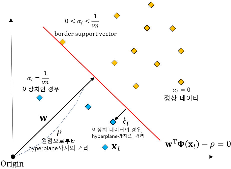
데이터를 N차원 좌표측으로 표현하고, 원점과의 거리를 기준으로 초 평면을 그어 Classification하는 방법

비지도 학습: One-Class SVM은 정상 데이터만을 사용하여 학습되며, 이상치의 라벨이 필요하지 않습니다.
커널 사용: One-Class SVM은 다양한 커널을 사용하여 비선형 데이터를 선형적으로 변환할 수 있습니다. 주로 ‘rbf’ 커널이 사용됩니다.
서포트 벡터: One-Class SVM은 서포트 벡터를 사용하여 초평면을 정의합니다. 서포트 벡터는 초평면에 가장 가까운 데이터 포인트입니다.
마진 최대화: One-Class SVM은 서포트 벡터와 초평면 사이의 거리, 즉 마진을 최대화하는 초평면을 찾습니다.

장점
- 비지도 학습이 가능
- 적은 데이터량으로 학습해도 일반화 능력이 좋음
단점
- 데이터 량이 늘어날 수록 연산량이 크게 증가함
- 데이터 스케일링에 민감함
- Hyper parameter를 잘 조절해야 함

  
from sklearn.svm import OneClassSVM

# kernel: 사용할 커널 타입을 지정합니다. ('linear', 'poly', 'rbf', 'sigmoid', 'precomputed')
# nu: 훈련 오류의 비율 상한 및 서포트 벡터의 비율 하한입니다. (0, 1] 구간이어야 합니다.
# gamma: 'rbf', 'poly', 'sigmoid' 커널의 계수입니다. 'scale'은 1 / (n_features * X.var()), 'auto'는 1 / n_features를 사용합니다.
clf = OneClassSVM(kernel='rbf', nu=0.1, gamma='auto')
clf.fit(X)

y_pred = clf.predict(X)

  
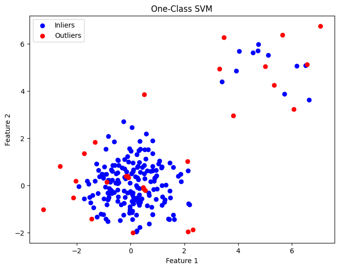
plt.figure(figsize=(8, 6))
plt.scatter(X[y_pred == 1, 0], X[y_pred == 1, 1], c='blue', label='Inliers')
plt.scatter(X[y_pred == -1, 0], X[y_pred == -1, 1], c='red', label='Outliers')
plt.title('One-Class SVM')
plt.xlabel('Feature 1')
plt.ylabel('Feature 2')
plt.legend()
plt.show()

참고자료

Data Analysis, Anomaly Detection

Isolation Forest 이상 탐지

Extended Isolation Forest 이상 탐지

One-Class SVM 이상 탐지

인기 태그