[Project] MLflow 만들기

MLflow

MLflow는 머신 러닝 실무자와 팀이 머신 러닝 프로세스의 복잡성을 처리하는 데 도움을 주기 위해 특별히 구축된 오픈 소스 플랫폼입니다. MLflow는 머신 러닝 프로젝트의 전체 수명 주기에 초점을 맞춰 각 단계가 관리 가능하고 추적 가능하며 재현 가능하도록 보장합니다. 즉, 머신러닝 학습과 관련된 전반적인 lifecycle을 지원하는 라이브러리입니다.

EDA

import pandas as pd
import numpy as np
import matplotlib.pyplot as plt
import plotly.graph_objects as go
%matplotlib inline

 

데이터 셋은 다음 링크에서 받을 수 있습니다.

https://www.kaggle.com/datasets/anikannal/solar-power-generation-data

 

generation = pd.read_csv("./data/Plant_1_Generation_Data.csv")
weather = pd.read_csv("./data/Plant_1_Weather_Sensor_Data.csv")

generation.head()

	DATE_TIME	PLANT_ID	SOURCE_KEY	DC_POWER	AC_POWER	DAILY_YIELD	TOTAL_YIELD
0	15-05-2020 00:00	4135001	1BY6WEcLGh8j5v7	0.0	0.0	0.0	6259559.0
1	15-05-2020 00:00	4135001	1IF53ai7Xc0U56Y	0.0	0.0	0.0	6183645.0
2	15-05-2020 00:00	4135001	3PZuoBAID5Wc2HD	0.0	0.0	0.0	6987759.0
3	15-05-2020 00:00	4135001	7JYdWkrLSPkdwr4	0.0	0.0	0.0	7602960.0
4	15-05-2020 00:00	4135001	McdE0feGgRqW7Ca	0.0	0.0	0.0	7158964.0

weather.head()

	DATE_TIME	PLANT_ID	SOURCE_KEY	AMBIENT_TEMPERATURE	MODULE_TEMPERATURE	IRRADIATION
0	2020-05-15 00:00:00	4135001	HmiyD2TTLFNqkNe	25.184316	22.857507	0.0
1	2020-05-15 00:15:00	4135001	HmiyD2TTLFNqkNe	25.084589	22.761668	0.0
2	2020-05-15 00:30:00	4135001	HmiyD2TTLFNqkNe	24.935753	22.592306	0.0
3	2020-05-15 00:45:00	4135001	HmiyD2TTLFNqkNe	24.846130	22.360852	0.0
4	2020-05-15 01:00:00	4135001	HmiyD2TTLFNqkNe	24.621525	22.165423	0.0

generation.info()

<class 'pandas.core.frame.DataFrame'>
RangeIndex: 68778 entries, 0 to 68777
Data columns (total 7 columns):
 #   Column       Non-Null Count  Dtype  
---  ------       --------------  -----  
 0   DATE_TIME    68778 non-null  object 
 1   PLANT_ID     68778 non-null  int64  
 2   SOURCE_KEY   68778 non-null  object 
 3   DC_POWER     68778 non-null  float64
 4   AC_POWER     68778 non-null  float64
 5   DAILY_YIELD  68778 non-null  float64
 6   TOTAL_YIELD  68778 non-null  float64
dtypes: float64(4), int64(1), object(2)
memory usage: 3.7+ MB

weather.info()

<class 'pandas.core.frame.DataFrame'>
RangeIndex: 3182 entries, 0 to 3181
Data columns (total 6 columns):
 #   Column               Non-Null Count  Dtype  
---  ------               --------------  -----  
 0   DATE_TIME            3182 non-null   object 
 1   PLANT_ID             3182 non-null   int64  
 2   SOURCE_KEY           3182 non-null   object 
 3   AMBIENT_TEMPERATURE  3182 non-null   float64
 4   MODULE_TEMPERATURE   3182 non-null   float64
 5   IRRADIATION          3182 non-null   float64
dtypes: float64(3), int64(1), object(2)
memory usage: 149.3+ KB

 

각 DATE_TIME이 Object이기에 datetime type으로 변환시킵니다.

 

generation['DATE_TIME'] = pd.to_datetime(generation['DATE_TIME'], dayfirst=True)
weather['DATE_TIME'] = pd.to_datetime(weather['DATE_TIME'], dayfirst=True)

C:\Users\PC\AppData\Local\Temp\ipykernel_24200\2802134372.py:2: UserWarning: Parsing dates in %Y-%m-%d %H:%M:%S format when dayfirst=True was specified. Pass `dayfirst=False` or specify a format to silence this warning.
  weather['DATE_TIME'] = pd.to_datetime(weather['DATE_TIME'], dayfirst=True)

generation_source_key = list(generation['SOURCE_KEY'].unique())
print('generation source key 갯수 :', len(generation_source_key))

generation source key 갯수 : 22

 

generation의 설비는 총 22개이므로 이 중 1개의 설비만을 분석하고자 합니다.

 

inv = generation[generation['SOURCE_KEY']==generation_source_key[0]]
mask = ((weather['DATE_TIME'] >= min(inv["DATE_TIME"])) & (weather['DATE_TIME'] <= max(inv["DATE_TIME"])))
weather_filtered = weather.loc[mask]

df = inv.merge(weather_filtered, on="DATE_TIME", how='left')
df = df[['DATE_TIME', 'AC_POWER', 'AMBIENT_TEMPERATURE', 'MODULE_TEMPERATURE', 'IRRADIATION']]
df.head()

	DATE_TIME	AC_POWER	AMBIENT_TEMPERATURE	MODULE_TEMPERATURE	IRRADIATION
0	2020-05-15 00:00:00	0.0	25.184316	22.857507	0.0
1	2020-05-15 00:15:00	0.0	25.084589	22.761668	0.0
2	2020-05-15 00:30:00	0.0	24.935753	22.592306	0.0
3	2020-05-15 00:45:00	0.0	24.846130	22.360852	0.0
4	2020-05-15 01:00:00	0.0	24.621525	22.165423	0.0

df.info()

<class 'pandas.core.frame.DataFrame'>
RangeIndex: 3154 entries, 0 to 3153
Data columns (total 5 columns):
 #   Column               Non-Null Count  Dtype         
---  ------               --------------  -----         
 0   DATE_TIME            3154 non-null   datetime64[ns]
 1   AC_POWER             3154 non-null   float64       
 2   AMBIENT_TEMPERATURE  3154 non-null   float64       
 3   MODULE_TEMPERATURE   3154 non-null   float64       
 4   IRRADIATION          3154 non-null   float64       
dtypes: datetime64[ns](1), float64(4)
memory usage: 123.3 KB

df_timestamp = df[["DATE_TIME"]]
df_ = df[["AC_POWER", "AMBIENT_TEMPERATURE", "MODULE_TEMPERATURE", "IRRADIATION"]]

 

모델을 train과 validation으로 분리합니다.

 

train_prp = .6
train = df_.loc[:df_.shape[0]*train_prp]
test = df_.loc[df_.shape[0]*train_prp:]

from sklearn.preprocessing import MinMaxScaler
scaler = MinMaxScaler()
X_train = scaler.fit_transform(train)
X_test = scaler.transform(test)
X_train = X_train.reshape(X_train.shape[0], 1, X_train.shape[1])
X_test = X_test.reshape(X_test.shape[0], 1, X_test.shape[1])
print(f"X_train shape: {X_train.shape}")
print(f"X_test shape: {X_test.shape}")

X_train shape: (1893, 1, 4)
X_test shape: (1261, 1, 4)

Model design

import torch
import torch.nn as nn
from torch.utils.data import DataLoader, TensorDataset

LSTMAutoencoder라는 모델을 사용해서 시계열 이상탐지를 진행하고자 합니다. 위 자세한 사항은 Unsupervised Learning of Video Representations using LSTMs을 참고하시면 됩니다.

추후에 LSTMAutoencoder를 정리해보겠습니다.

class LSTMAutoencoder(nn.Module):
    def __init__(self, seq_len, n_features):
        super(LSTMAutoencoder, self).__init__()
        # 인코더
        self.encoder_lstm1 = nn.LSTM(input_size=n_features, hidden_size=16, batch_first=True)
        self.encoder_lstm2 = nn.LSTM(input_size=16, hidden_size=4, batch_first=True)

        # 디코더
        self.decoder_lstm1 = nn.LSTM(input_size=4, hidden_size=4, batch_first=True)
        self.decoder_lstm2 = nn.LSTM(input_size=4, hidden_size=16, batch_first=True)
        self.decoder_output = nn.Linear(16, n_features)
        self.seq_len = seq_len

    def forward(self, x):
        x, _ = self.encoder_lstm1(x)
        x, (h_n, _) = self.encoder_lstm2(x)

        x = h_n.repeat(self.seq_len, 1, 1).permute(1, 0, 2)

        x, _ = self.decoder_lstm1(x)
        x, _ = self.decoder_lstm2(x)
        x = self.decoder_output(x)
        return x

def model_traning(epochs, learning_rate, dataloader):
    model = LSTMAutoencoder(seq_len=X_train.shape[1], n_features=X_train.shape[2])
    criterion = nn.L1Loss()
    optimizer = torch.optim.Adam(model.parameters(), lr=learning_rate)

    for epoch in range(epochs):
        model.train()
        epoch_loss = 0
        for batch_x, _ in dataloader:
            output = model(batch_x)
            loss = criterion(output, batch_x)
            optimizer.zero_grad()
            loss.backward()
            optimizer.step()
            epoch_loss += loss.item()

        if (epoch+1) % 10 == 0:
            print(f"Epoch {epoch+1}/{epochs}, Loss: {epoch_loss:.4f}")

    return model

Model Optimization

mlflow를 사용하기 위해서는 mlflow ui를 실행했을 때, 사용되는 URI를 입력합니다.

mlflow ui

실행하기 이전에 위 명령어를 실행시켜야 합니다.

import mlflow
from mlflow.data.pandas_dataset import PandasDataset

mlflow.set_tracking_uri("http://127.0.0.1:5000")
# mlflow.create_experiment("mlflow-lab")

mlflow ui에서 Experiments라고 실험을 분리할 수 있습니다. 저는 mlflow-lab에 분리하여 진행하겠습니다.

mlflow.set_experiment("mlflow-lab")

<Experiment: artifact_location='mlflow-artifacts:/148508904301274675', creation_time=1742975277849, experiment_id='148508904301274675', last_update_time=1742975277849, lifecycle_stage='active', name='mlflow-lab', tags={}>

mlflow에서 모델을 돌릴때 그래프를 저장할 수 있습니다. 여러가지 모델을 돌리면 parameter마다 그래프가 어떻게 달라지는지 확인해볼 필요가 있기에 Visualization함수를 만듭니다.

def mae_visualization(scores):
    scores['datetime'] = df_timestamp.loc[1893:].values
    scores['real AC'] = test['AC_POWER'].values
    scores["loss_mae"] = (scores['real AC'] - scores['AC_POWER']).abs()
    scores['Threshold'] = 200
    scores['Anomaly'] = np.where(scores["loss_mae"] > scores["Threshold"], 1, 0)

    plt.figure(figsize=(12, 6))
    plt.plot(scores['datetime'], scores['loss_mae'], label='Loss (MAE)')
    plt.plot(scores['datetime'], scores['Threshold'], label='Threshold', linestyle='--')
    plt.title("Error Timeseries and Threshold")
    plt.xlabel("DateTime")
    plt.ylabel("Loss")
    plt.legend()
    plt.grid(True)
    plt.tight_layout()
    plt.savefig("./plot/model_mae_plot.png")

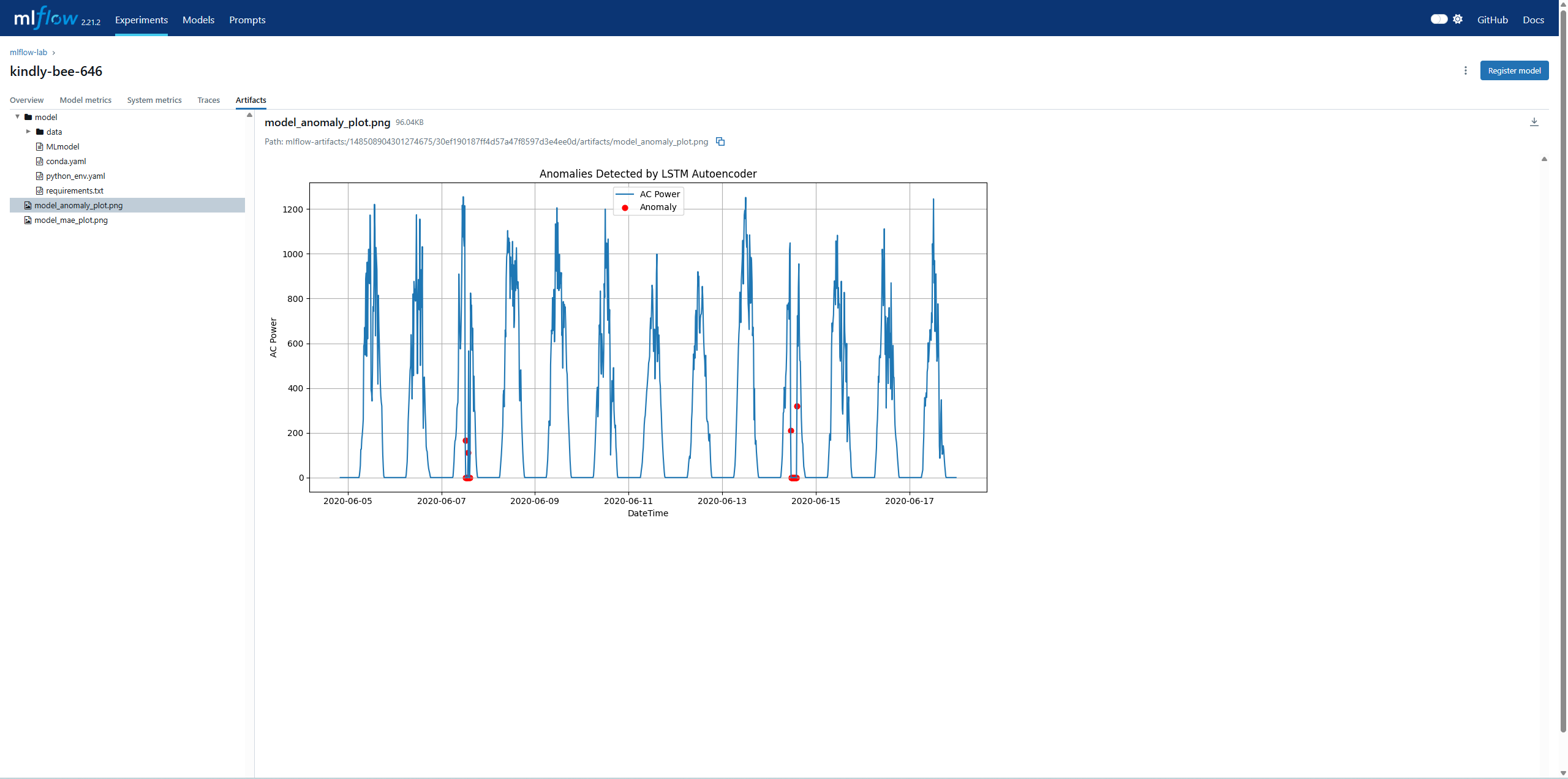
def anomaly_visualization(scores):
    anomalies = scores[scores['Anomaly'] == 1][['real AC']]
    anomalies = anomalies.rename(columns={'real AC': 'anomalies'})
    scores = scores.merge(anomalies, left_index=True, right_index=True, how='left')

    plt.figure(figsize=(12, 6))
    plt.plot(scores["datetime"], scores["real AC"], label='AC Power')
    plt.scatter(scores["datetime"], scores["anomalies"], color='red', label='Anomaly', s=40)
    plt.title("Anomalies Detected by LSTM Autoencoder")
    plt.xlabel("DateTime")
    plt.ylabel("AC Power")
    plt.legend()
    plt.grid(True)
    plt.tight_layout()
    plt.savefig("./plot/model_anomaly_plot.png")

with mlflow.start_run()을 사용하여 mlflow에 실행시킬 명령어를 작성합니다. 끝에는 mlflow.end_run()을 사용하여 mlflow가 끝났다는 것을 명시합니다.

for문을 통하여 설정한 parameter를 반복하여 최적의 paramter를 찾을 수 있습니다.

또한, log_param을 설정하면 UI에서 각 paramter를 확인하고 비교할 수 있습니다. log_artifact를 설정하면 mlflow ui에서 데이터(이미지, csv등)을 각 모델에서 들어가 볼 수 있습니다.

이외의 다양한 mlflow 설정들은 https://mlflow.org/docs/latest/에서 확인할 수 있습니다.

for batch_size_search in [10,15,20]:
    for learning_rate_search in [0.001,0.01,0.1]:
        with mlflow.start_run(log_system_metrics=True):
            epochs = 10
            batch_size = batch_size_search
            learning_rate = learning_rate_search

            mlflow.log_param("epochs", epochs)
            mlflow.log_param("batch_size", batch_size)
            mlflow.log_param("learning_rate", learning_rate)

            X_tensor = torch.tensor(X_train, dtype=torch.float32)
            dataset = TensorDataset(X_tensor, X_tensor)
            dataloader = DataLoader(dataset, batch_size=batch_size, shuffle=True)

            # model traning
            model = model_traning(epochs, learning_rate, dataloader)

            # model evaluation
            model.eval()
            X_test_tensor = torch.tensor(X_test, dtype=torch.float32)
            with torch.no_grad():
                X_pred = model(X_test_tensor).numpy()
            
            X_pred = X_pred.reshape(X_pred.shape[0], X_pred.shape[2])
            X_pred = scaler.inverse_transform(X_pred)
            X_pred = pd.DataFrame(X_pred, columns=train.columns)
            X_pred.index = test.index

            # visualization
            mae_visualization(X_pred)
            anomaly_visualization(X_pred)

            mlflow.log_metric("anomaly cnt", len(X_pred[X_pred['Anomaly'] == 1]))

            mlflow.log_artifact("./plot/model_mae_plot.png")
            mlflow.log_artifact("./plot/model_anomaly_plot.png")

            mlflow.pytorch.log_model(model, "model")

mlflow.end_run()

MLflow UI를 확인해보면

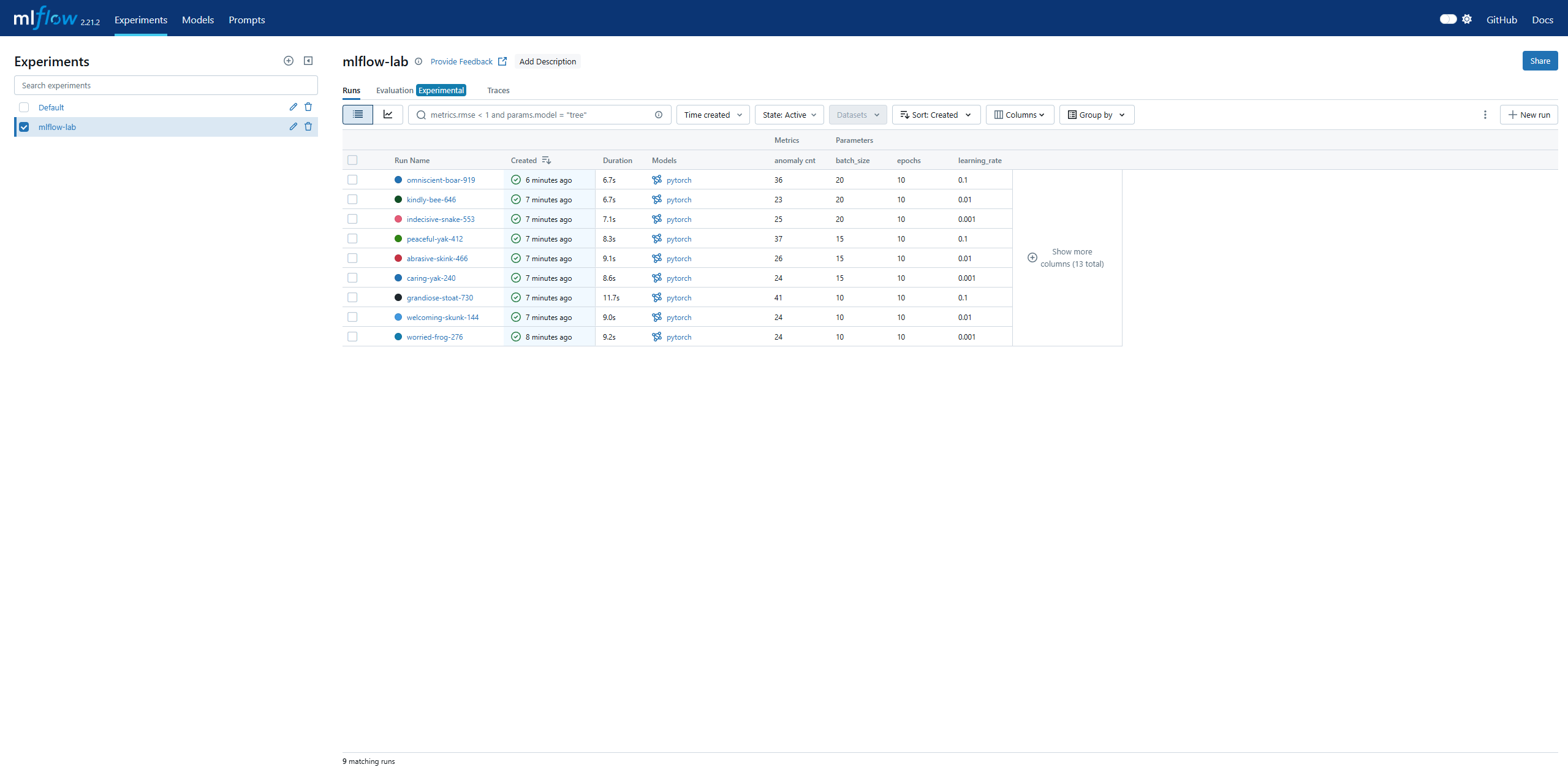
설정한 paramter들로 학습된것을 확인할 수 있습니다. log_paramter에 설정한 값은 각 오른쪽을 통해 확인할 수 있습니다. 만약 accuracy, precision, recall, fl score등을 넣고 싶으면 log_matric에 설정하면 확인할 수 있습니다. 이를 통해서 가장 잘 맞춘 모델의 paramter를 확인할 수 있습니다.

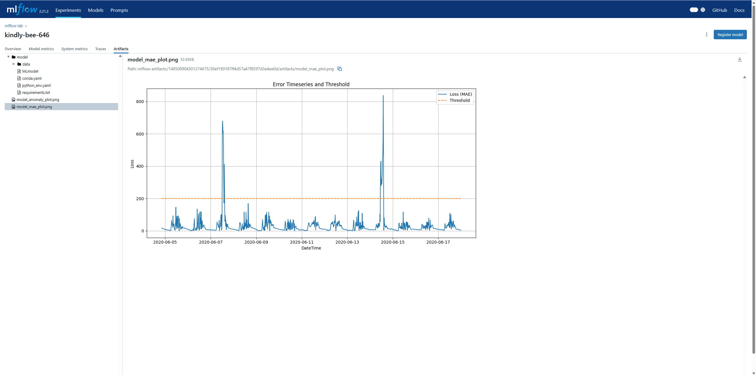
Run Name을 클릭하여 상단의 Artifacts를 확인하면 저장한 그래프를 확인할 수 있습니다.

 

참고자료

• https://arxiv.org/abs/1502.04681
• https://mlflow.org/docs/latest/